TEMSIM

Usage

The package is made of several programs which can be run (for example in the case of Silicon with incident beam in the $[110]$ direction) with the following commands :

cat Si110A.in | temsim/atompot
cat Si100_mulslice.in | temsim/mulslice
cat Si100_autoslic.in | temsim/autoslic

where :

Program	Input	Output	Description
atompot	slice.dat slice.in	slice.tif	computes the projected potential $V_z(x,y)$
mulslice	slice.tif name.in	name_mulslice.tif	periodic multislice simulation
autoslic	coords.xyz name.in	name_autoslic.tif	non periodic multislice simulation

Python interface

A simple Python interface can generate the input decks (*.in), run temsim and postprocess the results. Type python3 -c "from multislice import Multislice; help(Multislice)" for command line help. The doc is built with : make multislice_doc.

datafile generation

The .xyz coordinate file can be automatically generated from a structure file (pdb,cif,built-in,... imported with crystals library) using make_xyz. The orientation is controlled by providing the incident beam direction n in lattice coordinates :

make_xyz(name='dat/Lithium',compound='Li',n=[1,1,1],fmt='%.4f')

BCC[001]	BCC[110]	BCC[111]

deck generation

The following example generates the decks for an autoslic simulation located in relative path Silicon/Si110 which would contain the coordinates file *.xyz. The simulation is setup with $6\times 6$ transverse unit cells repeated $N_z=40$ times along beam direction (which results in a total thickness $T=c_zN_z$ ), a sampling $512\times 512$ and a slice thickness $\Delta z=1.3575A$ .

from multislice import Multislice
multi=Multislice('Silicon/Si110',mulslice=False,
                repeat=[6,6,40],slice_thick=1.3575,NxNy=[512,512])

running a simulation

The simulation can then be run(remotely if ssh provided) and monitored using the generated input decks or directly through the interface with :

multi.run(ssh='')
multi.check_simu_state(ssh='')
multi.print_log()

post process

Once the simulation is over, post-process can be performed. Plotting the beam intensities as function of thickness and displaying the diffraction pattern as :

multi.beam_vs_thickness(bOpt='f') #force re postprocess
multi.pattern()                   #diffraction pattern

utilities

The library scattering can be used to compute the scattering factor and structure factor. This can be useful for analysing the results. Here for example the structure factor of Silicon is calculated as :

from scattering.structure_factor import *
from crystals import Crystal
N,sym = 4,False
#
# get info for Silicon from crystals library
Si,Z = Crystal.from_database('Si'),14                               
lat_vec   = Si.reciprocal_vectors                                   # get reciprocal lattice vectors
pattern   = np.array([list(a.coords_fractional)+[a.atomic_number] for a in crys.atoms])
hkl,Fhkl  = structure_factor3D(pattern,lat_vec,hklMax=N,sym=sym)    # compute structure factor up to 4th order in each direction
Shkl      = np.abs(Fhkl)**2                                         # Compute intensities
plot_structure3D(hkl,Shkl)                                          # plot in 3D

atompot

Computes the projected potential of a slice.

Input deck

Contains the parameters :

#pot.in
srta.dat      # structure file (for SrTiO3 here)
srtapot.tif   # output image file(to feed to multislice)
512 512       # real space pixel Nx,Ny
8 8 1         # replicate unit cell
n             # no thermal displacement

Slice file

where the files describing the slices srta.dat and srtb.dat read :

################# Slices for SrTiO3 ###################
#######################################################
# Si110A.dat
  3.9051 3.9051 1.9525    #lattice constants ax,bx and slice thickness cz
0                         #no symmetry operation
38                        # Strontium Z=38
  1.0000 0.0000 0.0000    #   corner of the cell

8                         # Oxygen
  1.0000 0.5000 0.5000    #   centre of the cell
#######################################################
# strb.dat
  3.9051 3.9051 1.9525    #lattice constants ax,bx and slice thickness cz
0                         #no symmetry operation
22                        #1 Titanium atom Z=22
  1.0000 0.5000 0.5000    #   centre of the cell

8                         # 2 Oxygen atom Z=8
  1.0000 0.5000 0.0000    #   edge of the cell
  1.0000 0.0000 0.5000    #   edge of the cell

Variables

iz : atomic number
nsx,nsy : $(N_x,N_y)$ cell to replicate
featom : atomic scattering factor of atom iz from Gaussian+Lorentzian fits at $k^2$ , $f^e_j(k^2)=\sum_{i=1}^{3}a_i/(k^2+b_i) + c_ie^{-d_ik^2}$
scamp : scattering amplitude structure factor due to atoms iz, $\sum_{j} e^{i\bb k\cdot\bb r_j}$
cpix : projected potential of the slice $V(x,y)=\int_{Slice} V(x,y,z')dz' =\mathcal F_{2D}^{-1} \left( \sum_{iz} f_{iz}^e(k^2)\sum_{j\in j(iz)}e^{i\bb k\cdot\bb r_j}\right)$

Code

//atompot.cpp
int main()
  //get parameters
  k2max = 1.0 / max(2*ax/nx,2*by/ny)^2;
  rx2 = (1.0/ax)^2;ry2 = (1.0/by)^2;
  scale = ( ((double)nx)*((double)ny) ) /(ax*by);
  for( i=0; i<=n_atom_types; i++)
    ns = sscanf( cline, "%d", &iz);
    while( ReadLine( fp, cline, NCMAX, filein ) > 2)
      ns = sscanf( cline, "%f %f %f %f", &occ[j], &x[j], &y[j], &wobble[j];
      natom++;    
    //projected potential contribution
    for( iy=0; iy<=iymid; iy++)
      ky2 = ky[iy]*ky[iy]*ry2;
      for( ix=0; ix<nx; ix++)   
        if(k2<k2max)
          k2 = kx[ix] * kx[ix]*rx2 + ky2;
          fe = scale * featom( iz, k2 );
          scamp( kx[ix], ky[iy], &scampr, &scampi ) ;
          cpix(ix,iy) += scampr*fe;
  cpix.ifft(); // inverse fourier transform

//atompot.cpp
void scamp( float kx, float ky, double scampr, double scampi )
  scalex = pi2*kx / ((double)nsx);scaley = pi2*ky / ((double)nsy);
  for( i=0; i<natom; i++)
    phasexr=phasexi=0;
    w1 = pi2 * kx * x[i];
    for( ixc=0; ixc<nsx; ixc++){
        w = w1 + ixc * scalex;
        phasexr += cos(w);
        phasexi += sin(w);
    w1 = pi2 * ky * y[i];
    for( iyc=0; iyc<nsy; iyc++)
        phaseyr=phaseyi=0;
        w = w1 + iyc * scaley;
        phaseyr += cos(w);
        phaseyi += sin(w);
    scampr += ( phasexr * phaseyr - phasexi * phaseyi ) * occ[i];
//slice.cpp
double featom( int Z, double k2 )
{
    if( feTableRead == 0 ) nfe = ReadfeTable();//fparams,
    sum = 0.0;
    //Lorentzians
    sum += fparams[Z][i]/( k2 + fparams[Z][i+1] );
    //Gaussians
    for( i=2 * nl; i<2 * (nl+ng); i+=2 )
        sum += fparams[Z][i] * exp( - k2 * fparams[Z][i+1] );
    return( sum );
}

mulslice

Input deck

Si110_mulslice.in contains multislice simulation parameters :

#mul.in
12(ab)      # stacking sequence
srtapot.tif # projected potential file a
srtbpot.tif # projected potential file b
srtrmul.tif # out binary file diffraction pattern
n           # include partial coherence
n           # resume from previous run
400         # incident beam energy in keV
0 0         # crystal tilt
0 0         # beam tilt
n           # record as a function of thickness

variables

wave : Transverse wave function $\Psi(x,y)$
trans[j] : Transmission function of layer $j$ , $e^{i\sigma v_{z,j}}$
prop[j] : Fourier transform of the propagator at layer $j$ , $e^{-i\pi\lambda\Delta z_j k^2}$
vz[j] : Projected potential of layer $j$ , $v_{z,j}=\int_{z_j}^{z_j+\Delta z_j} V(x,y,z')dz'$
cz[j] : Thickness of layer $j$ , $\Delta z_j$

Code

parsing parameter

ns = scanf("%s", filein[ilayer] );
lstart = askYN("Do you want to start from previous result");
if (lstart) ns = scanf("%s", filestart);
else ns = scanf("%g", &v0);
/*  calculate relativistic factor and electron wavelength */
mm0 = 1.0F + v0/511.0F;
wavlen = (float) wavelength( v0 );
scale = wavlen * mm0;
myFile.read( filein[ilayer])
vz=scale*myFile(ix, iy);
trans[ilayer].re(ix,iy) = (float) cos(vz);
trans[ilayer].im(ix,iy) = (float) sin(vz);
/*  calculate the total specimen thickness and echo */
cztot += cz[ layer[islice] ];
/*  calculate spatial frequencies and positions for future use */
rx = 1.0F/ax;rx2= rx*rx;
ry = 1.0F/by;ry2= ry*ry;
ixmid = nx/2;iymid = ny/2;
/*initialize wavefunction if resuming*/
if ( lstart == 1 ) {
  for( ix=0; ix<nx; ix++) for( iy=0; iy<ny; iy++) {
    wave0r[ix][iy] = myFile(ix,iy);
    wave0i[ix][iy] = myFile(ix+nx,iy);
    wave.re(ix,iy) = wave0r[ix][iy];
    wave.im(ix,iy) = wave0i[ix][iy];  
  }
  else
  // add incident beam tilt
  qx = btiltx / wavlen;qy = btilty / wavlen;
  wave.re(ix,iy) = (float) cos( t );
  wave.im(ix,iy) = (float) sin( t );
}
/* bandwidth limit the transmission function for anti-aliasing*/
const float BW= (2.0F/3.0F);
k2max = min(nx/(2.0F*ax),ny/(2.0F*by))
k2max *= BW * k2max;
/*set to zero outside sampling circle*/
trans[ilayer].fft();
for( ilayer=0; ilayer<nlayer; ilayer++) {
  for k2=kx+ky; if (k2 > k2max) trans[ilayer].re=trans[ilayer].im=0;
  trans[ilayer].ifft();
}
/*  calculate propagator function*/
scale = pi * cz[ilayer];
for( ix=0; ix<nx; ix++) {
    t = scale*( kx2[ix] * wavlen);
    propxr[ilayer][ix] = (float)  cos(t);
    propxi[ilayer][ix] = (float) -sin(t);
}
for( iy=0; iy<ny; iy++) {
    t = scale*( ky2[iy] * wavlen);
    propyr[ilayer][iy] = (float)  cos(t);
    propyi[ilayer][iy] = (float) -sin(t);
}

propagate

Propagation is performed as : $\begin{equation} \Psi_{n+1}(x,y)=FT^{-1}\Bigg\{ P(k^2,\Delta z_n)FT\Big(t_n(x,y)\Psi_n(x,y)\Big) \Bigg\} \end{equation}$

// mulslice.cpp
/* ------------------- coherent method --------------------*/
for( islice=0; islice<nslice; islice++ ){
  ilayer=layer[islice];
  wave = wave*trans[ilayer]; // transmit
  wave.fft();
  propagate(wave,
            propxr[ilayer], propxi[ilayer],propyr[ilayer],propyi[ilayer],
            kx2,  ky2,  k2max, nx, ny );
  wave.ifft();
  // transverse intensity integral
  sum = abs(wave)^2.sum()/(nx * ny)
  printf("layer = %c, integrated intensity = %f\n",cname[ilayer], sum );
}

autoslic

The program autoslic performs multislice simulation on non periodic structures.

Coordinates file

Input deck

Code

Parsing simulation setup

//autosliccmd.cpp
int main()
  autoslic aslice();
  cfpix pix,wave0,beams;
  aslice.lbeams = askYN("Do you want to record the (real,imag) value of selected beams vs. thickness");
  mm0 = 1.0F + v0/511.0F;
  wavlen = (float) wavelength( v0 );
  natom = ReadXYZcoord( filein.c_str(), ncellx, ncelly, ncellz,
    &ax, &by, &cz, &Znum, &x, &y, &z, &occ, &wobble,description );
  aslice.calculate(pix,wave0,natom,beams);
  if (lbeams)
    fp1.open(filebeam);
    fp1 << " (h,k) = " << hbeam[ib] << endl;
    fp1 << islice << beams.re(ib,islice) << beams.im(ib,islice) << endl;

Running the multislice simulation

//autoslic.cpp
void autoslic::calculate(cfpix &pix,cfpix &wave0, cfpix &depthpix,
                    natom, cfpix &beams,hbeam,kbeam)
  scale=1/(nx*ny);
  while (zlice<zmax)
    trlayer(trans);
    wave *= trans;
    wave.fft(); //reciprocal space
    if( (lbeams== 1) ) {
      beams.re(ib,islice-1) = scale*wave.re(hbeam[ib],kbeam[ib] );
      beams.im(ib,islice-1) = scale*wave.im(hbeam[ib],kbeam[ib] );
    }
    propagate(wave,propxr,propyr,propxi,propyi);
    wave.ifft();
    /*save intermediate intensities*/
    if (lcross){
      depthpix = wave.re*wave.re+wave.im*wave.im;
    }
    /*Return exit wave*/
    pix = wave;

Transmission function from projected potential

void autoslic::trlayer( const float x[], const float y[], const float occ[],const int Znum[], const int natom, const float ax, const float by,const float kev, cfpix &trans, const int nx, const int ny,const floatkx2[], const float ky2[],double *phirms, int *nbeams, const float k2max)
  scale = sigma(kev)/1000.0;scalex=ax/nx;scaley=by/ny;//sigma rad/V-A
//pragma omp parallel
  for( i=0; i<natom; i++)
    for( ix=nx1; ix<=nx2; ix++)
       rx = x[i] - ((double)ix) * scalex;
       for( iy=ny1; iy<=ny2; iy++)
          ry = y[i] - ((double)iy) * scaley;
          rsq = rx**2 + ry**2;
          vz += occ[i] * vzatomLUT( Znum[i], rsq );
  trans = exp(1J*scale*vz);
  /* bandwidth limit the transmission function */
  trans.fft();
  trans[k2<k2max] = 0;
  trans.ifft();

Real space atomic projected potential

Computing projected atomic potential from cubic spline interpolation using look up table coefficients.

splinx,spliny : Data projected atomic potential for spline interpolation
splinb,splinc,splind : spline coefficients

//slicelib.cpp
double vzatomLUT(int Z, double rsq)
  /*  generate a set of logarithmic r values */
  if (!spline_init)
    dlnr = log(RMAX/RMIN)/(NRMAX-1);
    for( i=0; i<NRMAX; i++)
        splinx[i] = (RMIN * exp( i * dlnr ) )^2;
  /* generate the spline coefficients from analytical projected potential expression */
  if (!nspline[iz]) //if this atomic number has not been called before do it once and for all
    for( i=0; i<NRMAX; i++)
        spliny[iz][i] = vzatom( Z, sqrt(splinx[i]));
    splinh( splinx, spliny[iz], splinb[iz],splinc[iz], splind[iz], NRMAX);
  /* now that everything is set up find the scattering factor by interpolation in the table   */
  vz = seval( splinx, spliny[iz], splinb[iz],
            splinc[iz], splind[iz], nspline[iz], rsq );

double vzatom( int Z, double r )
  const double al=150.4121417, ag=266.5985798;
  nfe = ReadfeTable(fparams);
  x = 2.0*pi*r;
  for( i=0; i<2*nl; i+=2 )
       suml += fparams[Z][i]* bessk0( x*sqrt(fparams[Z][i+1]) );
  x = (pi*r)**2;
  for( i=2*nl; i<2*(nl+ng); i+=2 )
      sumg += fparams[Z][i]*exp(-x/fparams[Z][i+1]) / fparams[Z][i+1];
  return( al*suml + ag*sumg );
//Compute

propagator

/*  multiplied by the propagator function */
//autoslic.cpp
void calculate()
  scale = pi*deltaz
  tctx = (float) (2.0 * tan(ctiltx));
  tcty = (float) (2.0 * tan(ctiltx));
  propxr[ix] = cos(scale*kx2*wavlen - kx[ix]*tctx)
  propxi[ix] = sin(scale*kx2*wavlen - kx[ix]*tctx)
  propyr[ix] = cos(scale*ky2*wavlen - ky[iy]*tcty)
  propyi[ix] = sin(scale*ky2*wavlen - ky[iy]*tcty)

//slicelib.cpp
void propagate(cfpix &wave,float* propxr, float* propxi, float* propyr, float* propyi,float* kx2, float* ky2, float k2max, int nx, int ny )
  for( ix=0; ix<nx; ix++)
    if( kx2[ix] < k2max )
      pxr = propxr[ix];
      pxi = propxi[ix];
      for( iy=0; iy<ny; iy++)
        if( (kx2[ix] + ky2[iy]) < k2max )
          pyr = propyr[iy];
          pyi = propyi[iy];
          wr = wave.re(ix,iy);   // real
          wi = wave.im(ix,iy);   // imag
          tr = wr*pyr - wi*pyi;
          ti = wr*pyi + wi*pyr;
          wave.re(ix,iy) = tr*pxr - ti*pxi;
          wave.im(ix,iy) = tr*pxi + ti*pxr;

Other programs

image formation effects (defocus,aberration,...) : temsmim/image
STEM(scanning => incident probe) : temsim/stemlic
STEM non periodic : temsim/autostem

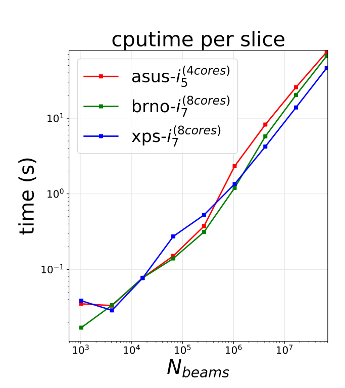
walltime

Kirkland	time per slice	time per slice per core